Showing posts with label Excel and Macros. Show all posts

Saturday, November 20, 2021

Match a Single Value in Multiple columns (Excel Tricks)

Hii All,

After a long long time I am back. I always want to share some new things which may be useful for some or the others like me but due to busy schedule in my job I do not get time for the same.

Anyways, today My friend asked a query that he want to match a Single Value in Multiple Columns of the source data and if it matches anywhere in the those columns it will bring the related cell value 

The below pic will clear more about his query.


So it is bit tricky as normally you can use Excel Match formula in a single column, But with the Excel IfError Formula you can solve the issue.


The formula is 

=INDEX(M5:M9,IFERROR(MATCH(D5,J5:J9,0),IFERROR(MATCH(D5,K5:K9,0),MATCH(D5,L5:L9,0))))


You can also download the example file by clicking below link.

Matching Single Value in Multiple Columns


Hope this post is useful and you can corelate a situation where you needed something like this.


Thanks...
 

Sunday, April 28, 2019

Tally Trial Balance Consolidation Utility in excel

Hello Friends,
Financial Year has ended recently and many of the accounts & finance professionals are ready for preparing the Balance Sheets.

Many companies have operations at multiple locations and they prepare the accounts accordingly and at the end consolidate the data and prepare the Final Accounts.

Normally the trial balances of each locations are consolidated and on that basis the Profit & Loss Accounts & Balance Sheets are prepared.

Sometimes, the consolidation of Trial Balance is lengthy, tricky and difficult part for the accounts professionals although its a simple process of summarizing the transactions.

So I am sharing an excel utility where upto 10 nos of Trial Balances (Tally Generated) can be consolidated within a minute.


The Excel utility is self explanatory, but some basic points are mentioned here: -
1. You need to export Group Names of each locations from tally and paste in this file.
2. You need to export Trial Balance of each location from tally and paste here.
3. You need to ensure that the Net Value should be Zero (0) .
    Because Debit = Credit, i.e. Debit-Credit = 0 (Otherwise there are some diff in the Trial Balance)


Hope this excel file be useful for your accounts work.


Click Here the download the Excel File


Saturday, June 24, 2017

Multipurpose excel utility - Useful for every manufacturing /trading business with statutory compliances

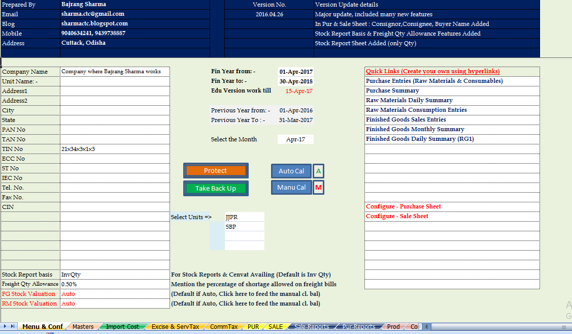
Today sharing one of my excel programming which has helped me to the maximum in my professional career and allowed me to work with accuracy, speedy reporting & controlling. And this also allowed to access most data within a single excel file and not to make the computer messy with thousands of useless sheets.

I have named it as operation sheet.
The time taken to design this is around 10 Years. Yes the first operation sheet was designed in the Year 2007 which was just for Purchase & Sales data with no auto error checks and gradually I included many functions which are inter linked with the basic functions of a business (i.e. Purchase & Sales)

** This sheet has been designed considering the Place of business is within Odisha and so far no effects of GST has been included.


The Usefulness about this sheets (as per me): -
1. Purchases & Sales Databases (with all relevant transaction details which we are not able to maintain or generate through tally/sap) Like Waybill, Transportation details, auto freight calculation, delivery date & weight, debit / credit notes bill wise, Quality (QC) details of each transactions , etc.
2. Taxation: - It is helpful for cenvat credits of excise duty, VAT Input.
3. Statutory Forms : - You can track which C-forms are pending / received / issued / receivable, etc
4. Statutory Payments :  You can enter the statutory Payment details and it will automatically show in the Excise / VAT charts and further you can cross check the liabilities.
5. You can enter the Consumption details (party wise also) , Production, Change the valuation method  (FIFO/LIFO/WAVG) and track which stocks are in your stock yard.
6. You can also enter the bill wise receipts from customers and track the outstanding. (Although for more details reports I use another sheet)
7. You can track that which bills are shown in returns and which are pending (assume you receive bills late, missed due to some reasons etc)
8. Freight Payments / Deductions : -Auto calculate the freight payable and track with accounts.

Many More functions has been added whichever and whenever I felt the importance of any thing I have tried to add that one.


Download this Excel Utility


Download this Excel Utility

Friday, April 22, 2016

How to Calculate Detention of Vehicles considering the complex Date & Time in excel


Some times it is difficult to calculate some cases which deals with Date & Time and calculating the Detention charges is one of them.


Please download the excel file (and do remember that it has been prepared on the basis the following basis.... which can be changed with the help of formulas)

https://drive.google.com/file/d/0Bw1qNoQ8YzHZY3E5VVl1SUduWm8/view?usp=sharing

Thursday, February 25, 2016

List out the details of files in a specified folder - automatically through excel without vba.

Hiii.
I was preparing a list of files (govt. forms) but it was difficult to manually copy the file name and paste into the excel sheet as there are more than 300 files in that folder.

After 8-10 copy paste I thought to do it automatically and the time saved is now used for writing this blog. LOL

Well, You can actually automatically list out the names of files in a specified folder into excel, assume that in a school there are 1000 students and their admit card is in one folder.. and for some reasons you need to list out it into an excel sheet.. So how you will do it...........


Here is a simple and superb way to do that........

These are the steps assuming your folder name is "Admit Card" and it is stored in D Drive...
1. Open a new excel file
2. Click on "Formulas" and then "Define Naem"
3. In the name field type AdmitCardList   (You can put any other name also)
4. In refers to Column type: - =FILES("D:\Admit Card\*.*")&T(NOW()) and press OK.
5. Now In your sheet 1 and cell A1 type or copy paste this formula
 =IF(ISERROR(INDEX(AdmitCardList,ROW()-1)),"",INDEX(AdmitCardList,ROW()-1))

and drag it downwards and you will see that your list is automatically updating.....


Hope the above can save your time too in case of huge data working and you will smile remembering this post...

Byee............... If you require the excel file, please inform........

Saturday, November 15, 2014

Some Useful tips on MS Excel - Specially for those who are using Excel

Quick Help
To get quick help on any menu item push Shift+F1 and click the menu item
Insert Today's Date
To insert Today's date push Ctrl+; (semicolon)
Insert Current Time
To insert the current time push Ctrl+Shift+: (Colon)
Show the Paste Function (Function Wizard)
Push Ctrl+F3
Show the GoTo dialog
Push F5
Show the Paste Names dialog
Push F3. This will only work if you have named ranges.
Name a Range
To name a selected range, click in the "Name box" (far left on the formula bar) and type a one word name.
Go To a Named Range
To go to a named range select it from the "Name box" (far left of the formula bar). Or push F5.
Edit a Named Range
To delete or edit a named range go to Insert>Name>Define or Push Ctrl+F3.
Headings as Range Names
Highlight your range including the headings and go to Insert>Name>Create or push Ctrl+Shift+F3.
Named Formula
To make a Name refer to a constant formula e.g. "TaxRate", go to Insert>Name>Define and type TaxRate in the "Names in Workbook" box and 36% in the "Refers To". Now enter =(10*TaxRate) anywhere on the Worksheet.
Named Range List
To obtain a list of all Named Ranges and where they refer, select any blank cell (make sure you have no data underneath or 1 column over) and go to Insert>Name>Paste then Paste List.
Nested Formulas
To help write nested formulas (more than 1 formula in a single cell) use the "Paste Function" i.e. Insert>Function or Shift+F3. Select the function that you need, enter the reference, number or text then select the drop arrow to the left of the formula bar to add more Formulas. Doing it this way ensures all your parentheses are in the correct places.
Debugging Formulas
To troubleshoot complex formulas select the cell containing it and then click the = (Equal sign) to the left of the formula bar, this will activate the "Paste Function". To step through your formula simply click in the part of the formula you want to debug.
Personal Help
To add your own text to any of the Office Assistants help files, push F1, enter your question then open the file. Go to Options>Annotate and type in your own text then click OK. You will now notice a paperclip symbol next to the heading, this will let you know that you have added your own Help in a way you will understand.
Different Help
Sometimes the Office Assistant is not very helpful to your needs, so try the "Context and Index" help by either clicking Help>Context and Index or selecting "Help Topics" from any "Help" file.
Customizing Toolbars
Right click on any Toolbar and select "Customize" or push Ctrl+Shift+F10 twice then "Customize". Now click the "Commands Tab" and drag menu items both on and off the Toolbars. If things get a bit messy simply click the "Toolbars" tab and click "Reset". This will return all menu items to their default.
Quick Charts
To create quick charts, click anywhere within your data and push F11.
Worksheet Template
Set up your Worksheet how you want it e.g. formatting, formulas etc then delete all other sheets in the Workbook. Now go to File>Save or Alt+F2 and select "Template (*.xlt)" from the "Save as Type". Type a name and click "Save" Now right click on the sheet tab and select Insert you should see yourTemplate sheet.
Secret Menu
Click in any cell, then move your mouse pointer over any border of the cell until the mouse pointer changes to an arrow, right click and drag to it's destination and then release.
Secret Menu 2
Place a date in any cell, then move your mouse pointer over the bottom right corner of the cell (Fill handle) until the mouse pointer changes to a small black cross. Now right click and drag to any cell and release.
Quick Cell Move
Click in the cell(s) then move your mouse pointer over any border until the mouse pointer changes to an arrow, left click and drag to it's destination and then release.
Quick Cell Copy
Click in the cell(s) then move your mouse pointer over any border until the mouse pointer changes to an arrow, left click and hold down the Ctrl key and drag to it's destination and then release.
Change Formulas to Values
Click in the cell(s) with the formula(s) then move your mouse pointer over any border until the mouse pointer changes to an arrow, right click and drag to the next cell, now still holding down the right mouse button drag back to where you started and release. Now select Copy here as values only.
Quick List
To quickly copy down the contents of a cell that has a list in the column to the left or right of it, simply click in the cell you want to copy and then Double click the Fill handle (little black square on the bottom right of the cell).
Fill Blank Cells Within a List
Let's say you have a list of entries in column A and within the list you have many blank cells. Here is a quick way to fill those blanks with the value of the cell above. Highlight column A, then push Ctrl+G and click Special then check the Blanks option and click OK. Now push Equals (=) then the Up arrow and finally holding down the Ctrl key push Enter.
Auto Fill
To fill a series across columns or down rows type January or Jan in any cell and place your mouse pointer over the bottom right corner of the cell (Fill handle) until the mouser pointer changes to a small black cross. Left click and drag down or across. This can also be done with Numbers, Weekdays, Quarters or any text that ends in a number e.g. Day1.
Custom Auto Fill
Type your list across columns or down rows. Now go to Tools>Option and select the "Custom Lists" tab. Click the collapse dialog box to the right of the "Import list from cells" box, highlight your range, click the expand dialog and then click "Import". Or type your entries in the "list Entries" box.
Adding Text to Formulas
To show a formula result and text or number(s) in the same cell type a & (Ampersand) after the formula then your text/number(s).
Adding Hidden Text to Formulas
Imagine you have a formula like: =$2018+$1056-4*$120. When you initially wrote it you knew what each number represented, but you come back later and can't remember. Add a hidden note to your formula by using the N() formula i.e. =$2018+$1056-4*$120+N("My Wage+Bonus-4 weekly loan repayments"). The N() function will convert text to zero.
Custom Format
You can format a cell to show any number or text without changing it's real value using "Custom Format". To see this type the number 20 in any cell then go to Format>Cells or push Ctrl+1. Select the "Number" tab and then select "Custom." Using any one of the pre-defined formats type "Twenty" (without quotations) or any text and then click "OK". To test it use the cell in any formula.
No More Chart Gaps
If you have a chart that is plotting empty text ("") or 0 (zero) from a formula then instead of using "" or 0 if the formula is False try using "#N/A" (without the quotations) or the formula =NA(). Or you can hide the Row(s) or Column(s). Either way Excel won't plot #N/A or hidden Rows or Columns.
My List
If you have a long list of Text with no blank cells between and you want to see a preview of what is in your list. Click in any cell within your list then right click and select "Pick from list", If you select one of the entries, Excel will insert it in the cell for you.
Remove Blank Rows
Highlight your range and go to Edit>Go to>Special and select "Blanks" then "Ok" now go toEdit>Delete or Ctrl+Shift+= (equal) and then select "Entire row" from the "Delete" dialog and click "Ok".
Sort Out Blank Rows
The quickest way to remove all blank rows is to select you range then go to Data>Sort.
See Formula cells
If you have a sheet full of formulas and you want to identify these cells at a glance go to Edit>Go to>Special and select "Formulas" then click "OK". Now go to Format>Cells or Ctrl+1 and select the "Patterns" tab and choose a color.
En Masse Changes
To make changes to more than one worksheet at the same time select one of the sheets, hold down your Ctrl key and click on each sheet name tab. Now any data entered one sheet will also be entered on the other(s). When you have finished right click on any of the sheet name tabs and select "Ungroup sheets".
En Masse Changes 2
Another way to have changes on one worksheet reflected on other sheets is to make all the changes you want on one sheet then hold down your Ctrl key and select the other sheet tabs. Go to Edit>Fill>Across Worksheets and Excel will give you 3 choices of what to copy to the other sheets i.e. "All", "Contents" or "Formats".
Worksheet Copy
Select the sheet name tab then hold down your Ctrl key and simply drag it to the position you want it.
Paste Reference
An easy way to reference another cell is to select the cell you wish to reference then right click and   select Copy or Ctrl+C then select the cell you want the reference in, right click again and select "Paste Special" then click "Paste Link"
Absolute/Relative Toggle
If you have a formula you want to make absolute or relative then double click in the cell or F2 then place the insertion point anywhere in the cell address and push F4 1, 2 or 3 times.
Repeat
To repeat an operation push F4
Undo
To undo an operation push Ctrl+Z
Linked Picture
A good alternative to a textbox or any shape is a linked picture that reflects any changes made to its reference. To make one, copy your cell(s), select the destination cell and holding down your Shift key go to Edit<Paste Picture Link.
Run a Macro by Clicking a Cell
This is possible with use of VBA but let's face it most people don't know VBA so here is an easy way. Select the cell you want to run the macro and hold down your Shift key and go to Edit>Copy Picture then select "As shown on screen" from the "Copy Picture" dialog then hold down your Shiftkey again and go Edit and click "Paste Picture". Now right click on the cell picture and "Assign Macro".
Non Formula Result
Sometimes you just want the result from the Sum, Average, Min, Max etc from a group of cells without typing a formula in a cell. Excel allows you to do this very easily, first highlight the cells you want to evaluate then right click on the "Status Bar" and select the function you want and your result will be displayed in the "Status Bar".
Reduce File Size
When you have a workbook that is very large in size you can reduce this dramatically by saving the file as "Microsoft Excel Workbook (*.xls)" as apposed to "Microsoft Excel 5/95 Workbook (*.xls)". In other words avoid saving as multiple versions whenever possible. Also click here for much more details and other methods.
Cell Navigation
To move through a group of cells that you are working with without going outside the range highlight the group of cells and then use the "Enter" key to move through them.
Quick Formula Syntax
When writing formulas for Excel sometimes you just need a quick reminder of the formula syntax. In this is the case then type an equal sign followed by the function name and push Ctrl+Shift+A. For Example typing =Vlookup and then pushing Ctrl+Shift+A will give you: =vlookup(lookup_value,table_array,col_index_num,range_lookup). The non-bolded arguments are optional.
How to copy formulas without the reference changing
This can be achieved by either pressing F2 and then highlighting the formula, Copy, Enter then paste to destination. Or doing the same in the Formular bar. However, this is not much good for large amounts of data, so try this: Select the range of cells with Formulae, use the Ctrl key for non-contiguous ranges. Now go to Edit>Replace and Replace = with #. Copy and paste to your location and then simply use Edit>Replace # with =
How to copy and transpose formulas without the reference changing
In cell A1 of sheet 2 put: =Sheet1!A1 now copy this down a max of 255 rows. Now with the formulas selected go to Edit>Replace and Replace = with #. Now copy, select cell B1, go to Edit>Paste special and choose Transpose. Delete Column "A" and with Row 1 selected go to Edit>Replace and Replace # with =
Turn a List Upside-Down
1. Copy the list to another location using Copy, Edit>Paste Special>Value.
2. Now select all data in the list, go to Tools>Options>Custom Lists.
3. Ensure the list address is in the "Import list from cells:" and click "Import".
4. Now go back to the column next to your list and in the top cell place the LAST entry from your list.
5. Now in the cell below, place the second last entry.
6. Select both cells and double click on the Fill Handle (small black square bottom right).
The list should now be reversed. You could now also sort you original list using Data>Sort>Options, nominate your list then sort!
Formula Errors
Whenever typing one of Excels functions (especially nested ones) into a cell always use lower case. This way when you push Enter Excel will capitalize only the names of the functions you have entered correctly.
Entering Named Ranges Into Formulas
When you write a formula, sometimes you want to use a Named Range as one of the arguments for the formula, but you cannot remember the name. In these times simply push F3 when you reach the argument that you want the Named Range in and Excel will display the Paste Name dialog. Click the name you want then OK.
Optional Function Arguments
Sometimes you may not be sure what arguments in a function are optional and which are not. If your using the Paste Function (Function Wizard) then the non-bolded arguments are optional.
Sort by more than 3 Columns
Excels sort feature only allows to nominate up to 3 columns to sort by, here is how to get around this. The key to this is sorting by the last key first and working back to the first key. Say you data is in Column A:E and you want to sort by A, B, C , D then E
1. Select all of Columns A:E
2. Go to Data>Sort> sort by C then by D then by E
3. Click Sort
4. Now again with Columns A:E selected
5. Go to Data>Sort> sort by A then by B
6. Click Sort
Printing Workbooks
If you have quite a few Workbooks to print, go to File>Open from within Excel, select the Workbook(s) uisng the Ctrl key, then right click and choose Print.


For any confusion or clarification, please feel free to comment.

Saturday, February 1, 2014

Spell the figures in Text (User defined formula) for Excel & VBA

Dear friends...
We often look / require a formula who can spell the figures in text.
In most of the reports we prepare we require to mentioned the figures / amount in text also. In some report this is mandatory to mention the same in text like bank deposit slips, any reports prepared for government department, etc etc.

But there is no such inbuilt formula in excel who can do this automatically.

** But now we can do the same with a UDF (user defined formula).

Let’s see how..

Copy and paste the following programme in the excel module. Module??? Ohhh.  For that following the following steps: -
1.        Right click on any sheet and select View Code
2.        In the top left of the window you will find the list of sheets
3.        Right click on any sheet and then click insert and then click module
4.        A module window will open.

Now copy paste the following codes into it.


Function SpellCurr(ByVal MyNumber, _
Optional MyCurrency As String = "Rupee", _
Optional MyCurrencyPlace As String = "P", _
Optional MyCurrencyDecimals As String = "Paisa", _
Optional MyCurrencyDecimalsPlace As String = "S")


          Dim Rupees, Paisa, Temp
          Dim DecimalPlace, Count
       
          ReDim Place(9) As String
          Place(2) = " Thousand "
          Place(3) = " Lakhs "
          Place(4) = " Crore "


          'String representation of amount.

          MyNumber = Trim(Str(MyNumber))
    
          'Position of decimal place 0 if none.
          DecimalPlace = InStr(MyNumber, ".")
         
          ' Convert Paisa and set MyNumber to Rupee amount.
          If DecimalPlace > 0 Then
              Paisa = GetTens(Left(Mid(MyNumber, DecimalPlace + 1) & _
                  "00", 2))
              MyNumber = Trim(Left(MyNumber, DecimalPlace - 1))
          End If

          If Len(Trim(Str(MyNumber))) Mod 2 = 0 Then
          MyNumber = "0" & Trim(Str(MyNumber))
          Else
          MyNumber = Trim(Str(MyNumber))
          End If

          Count = 1

          Do While MyNumber <> ""
          If Count = 1 Or Count > 7 Then
          Temp = GetHundreds(Right(MyNumber, 3))
          Else
          Temp = GetTens(Right(MyNumber, 2))
          End If
             
              If Temp <> "" Then Rupees = Temp & Place(Count) & Rupees
              If Len(MyNumber) >= 1 And Count < 2 Then
                  MyNumber = Left(MyNumber, Len(MyNumber) - 3)
              
              ElseIf Len(MyNumber) >= 1 And Count > 1 Then
              MyNumber = Left(MyNumber, Len(MyNumber) - 2)

              Else
             
                  MyNumber = ""
              End If
              Count = Count + 1

          Loop
           
            If MyCurrencyPlace = "P" Then
                Select Case Rupees
                    Case ""
                        Rupees = MyCurrency & "s" & " Zero"
                    Case "One"
                        Rupees = MyCurrency & " One"
                    Case Else
                        Rupees = MyCurrency & "s " & Rupees
                End Select
            Else
                Select Case Rupees
                    Case ""
                        Rupees = "Zero " & MyCurrency & "s"
                    Case "One"
                        Rupees = "One " & MyCurrency
                    Case Else
                        Rupees = Rupees & " " & MyCurrency & "s"
                End Select
            End If
           
          If MyCurrencyDecimalsPlace = "S" Then
                Select Case Paisa
                    Case ""
                        Paisa = " Only"
                    Case "One"
                        Paisa = " and One " & MyCurrencyDecimals & " Only"
                    Case Else
                        Paisa = " and " & Paisa & " " & MyCurrencyDecimals & "s Only"
                End Select
          Else
                Select Case Paisa
                    Case ""
                        Paisa = " Only"
                    Case "One"
                        Paisa = " and " & MyCurrencyDecimals & " One " & " Only"
                    Case Else
                        Paisa = " and " & MyCurrencyDecimals & "s " & Paisa & " Only"
                End Select
          End If
         
          SpellCurr = Rupees & Paisa

      End Function

      '*******************************************
      ' Converts a number from 100-999 into text *
      '*******************************************
     
      Function GetHundreds(ByVal MyNumber)
          Dim Result As String
          If Val(MyNumber) = 0 Then Exit Function
          MyNumber = Right("000" & MyNumber, 3)
          ' Convert the hundreds place.
          If Mid(MyNumber, 1, 1) <> "0" Then
              Result = GetDigit(Mid(MyNumber, 1, 1)) & " Hundred "
          End If

          ' Convert the tens and ones place.
          If Mid(MyNumber, 2, 1) <> "0" Then
              Result = Result & GetTens(Mid(MyNumber, 2))
          Else
              Result = Result & GetDigit(Mid(MyNumber, 3))
          End If
          GetHundreds = Result
      End Function

      '*********************************************
      ' Converts a number from 10 to 99 into text. *
      '*********************************************
     Function GetTens(TensText)

          Dim Result As String
          Result = ""           ' Null out the temporary function value.
          If Val(Left(TensText, 1)) = 1 Then   ' If value between 10-19...
              Select Case Val(TensText)
                  Case 10: Result = "Ten"
                  Case 11: Result = "Eleven"
                  Case 12: Result = "Twelve"
                  Case 13: Result = "Thirteen"
                  Case 14: Result = "Fourteen"
                  Case 15: Result = "Fifteen"
                  Case 16: Result = "Sixteen"
                  Case 17: Result = "Seventeen"
                  Case 18: Result = "Eighteen"
                  Case 19: Result = "Nineteen"
                  Case Else
              End Select
          Else                                 ' If value between 20-99...
              Select Case Val(Left(TensText, 1))
                  Case 2: Result = "Twenty "
                  Case 3: Result = "Thirty "
                  Case 4: Result = "Forty "
                  Case 5: Result = "Fifty "
                  Case 6: Result = "Sixty "
                  Case 7: Result = "Seventy "
                  Case 8: Result = "Eighty "
                  Case 9: Result = "Ninety "
                  Case Else
              End Select

              Result = Result & GetDigit _
                  (Right(TensText, 1))  ' Retrieve ones place.
          End If
          GetTens = Result
      End Function

      '*******************************************
      ' Converts a number from 1 to 9 into text. *
      '*******************************************
    
      Function GetDigit(Digit)
          Select Case Val(Digit)
              Case 1: GetDigit = "One"
              Case 2: GetDigit = "Two"
              Case 3: GetDigit = "Three"
              Case 4: GetDigit = "Four"
              Case 5: GetDigit = "Five"
              Case 6: GetDigit = "Six"
              Case 7: GetDigit = "Seven"
              Case 8: GetDigit = "Eight"
              Case 9: GetDigit = "Nine"
              Case Else: GetDigit = ""
          End Select
      End Function


Alternatively you can also download the code file by clicking the below link.
Click to download the Code file


Now save this and you have created a new formula for that particular file.

To use this you will have to type "=spellCurr(refer the cell address)"

Hope this is very simple and useful for all of you.

Cheers... Enjoy....